Overview

This hands-on tutorial has been developed to help researchers working with Gen3 data in Terra. The tutorial includes step-by-step instructions to cover the entire analysis process:

• How to link your Gen3 and Terra accounts

• How to find and export Gen3 data to a project workspace

• Understanding the structure of Gen3 data in Terra and how to make exported data more familiar

• How to run an interactive analysis in a Jupyter notebook

• How to configure and run a bulk analysis using workflow tools

Reading the documentation and following the step-by-step instructions will help familiarize you with Terra. The content on this page is available in a in Terra.

Tutorial Overview

A few caveats

• You should run through the steps below in order

• Note that you do not have to go through all of the steps in one sitting, only in the correct order

• Time estimates are conservative - many steps will take less time

How long does the tutorial take and how much does it cost?

Working through all of the tutorial steps should take just over an hour total (you can break it up and do at different times). The total computation cost of running both notebooks and the workflow will be less than $1.00.

Science overview

The tutorial models steps typical in a research journey using synthetic Gen3 phenotypic data and public-access 1,000 genomes genomic data. The data are stored in the BDC instance on the Gen3 platform. Phenotypic data are contained in the lab results and demographic nodes in Gen3 (and corresponding tables in Terra). The data are exported to Terra in the form of fifteen individual data tables connected to each other by UUIDs. The notebook section of the tutorial demonstrates how to select a subset of Gen3 tables you need - based on the data required for your analysis - and consolidate into one table with familiar subject ID conventions. This process of converting Gen3 data to a format that is more intuitive in Terra will be the same no matter what your final analysis. Section 7 covers how to run a bulk analysis workflow on the genomic data exported from Gen3. You would use the same process to do any bulk analysis on genomic data, such as aligning reads or calling variants.

Data disclaimer

The tutorial uses a synthetic, public-access dataset derived from 1,000 Genomes data and stored in the BDC instance in Gen3. For more information about how the synthetic data were generated, see .

Step-by-step Instructions

Set up tutorial workspace

Estimated time: one minute

Before you begin, you will need to create your own editable copy (clone) of this WORKSPACE to work in.

1. Click on the round circle with three dots in the upper right corner of the workspace.

2. Select "Clone" from the dropdown menu.

3. Rename your new workspace something memorable. It may help to write down or memorize the name of your workspace.

Follow-along worksheet

Work from your copy of this workspace following these . You can skim summaries of each step below.

Step 1. Link your Terra profile with Gen3

Estimated time: 2 minutes

If you haven't linked your Terra and Gen3 accounts yet, you need to follow these before you can analyze genomic data from Gen3 inside your Terra workspace.

Step 2. Access synthetic dataset on Gen3 platform

Estimated time: 5 minutes

This section walks through the process of accessing the public-access tutorial dataset (tutorial-synthetic_data_set_1) by going to the .

Step 3. Export data to workspace

Estimated time: 10 minutes - mostly exporting time

In this step you will practice exporting a Gen3 dataset to Terra. This process will be the same no matter what Gen3 data you are using. As part of this step, you will also learn about the structure of the exported data in a Terra workspace.

Step 4. Consolidate and format exported Gen3 data

Estimated time: 20 minutes

In this step, you will run the notebook 1-Consolidate-Gen3-data-in-Terra-tutorial. The tutorial notebook resolves some of the challenges of Gen3 data exported to Terra. In particular, it consolidates the tables that contain phenotypic data into one Terra table and reorganizes the tables and subject IDs to be more familiar. The notebook is also a good introduction to interactive analysis in a Jupyter notebook.

Notebook outline

• Set up the notebook environment

• Discover all of the metadata available from the Gen3 export

• Define and use a set of custom functions to

Step 5. Tidy up the consolidated table

Estimated time: 3 minutes

The consolidated table generated in Step 4 has almost 50 columns, including all of the Gen3 metadata from phenotypic data nodes. To help make the table more manageable to read without scrolling left and right, you can select the columns you want to see when you expand the table. This will allow you to focus on the information you need, without having to scroll across tens of columns. Your selections will persist even when you leave the workspace.

Step 6. Analyze consolidated data ("2-Analyze Gen3 data" notebook)

Estimated time: 15 minutes

In this step you will run the notebook 2-Analyze-consolidated-data-tutorial, which pulls data from the consolidated table into the notebook environment and does a bit of plotting analysis.

Notebook outline

• Import the consolidated phenotypic data from the new data table to the notebook compute environment

• This is where you would begin your project-specific analysis (in R or Python). We will explore the data by generating a few plots in the notebook.

Step 7. Run a workflow on genomic data

Estimated time: 5 minutes

Another mode of analysis in the Terra platform is bulk analysis with workflows. This mode is what you would typically use to do automated analysis steps such as processing genomic data. Bulk analysis uses workflow tools, which you can add to your workspace from another workspace, or by searching Dockstore or the Broad Methods Repository. In this step you will learn how to run a bulk analysis workflow to process genomic data in the the synthetic dataset from the Gen3 platform.

Next steps and additional resources

Congratulations! You have accessed and analyzed your first Gen3 data in Terra. Now that you have the basics of how to work with Gen3 data, here are some additional BDC and TOPMed resources to explore.

• workspace: This workspace includes the terra_data_util notebook, a notebook for unarchiving tar files, and eventually a vcf merge notebook

• Getting Started with Gen3

• GWAS template

Gen3 data overview

To understand what you will see when you export Gen3 data to a Terra workspace, it helps to first understand how the data is organized in Gen3. A diagram of the graph structure of the synthetic data in Gen3 is below on the left. Each box is a Gen3 data node and each line represents UUIDs connecting the metadata of the two nodes. Administrative nodes are purple, clinical data are in blue boxes, and genomic data are green boxes. When you export a project's data to a Terra workspace, each node in the graph gets imported as its own data table. Your data page will look like the figure on the right. The synthetic data in this tutorial is captured in 15 tables, corresponding to the 15 nodes in the graph structure.

Each data table includes all of the metadata fields associated with the Gen3 node, in alphabetical order. The lab_results table, for example, looks like this:

You might see from this example several features specific to the Gen3 data structure that can be challenging to work with in Terra:

• There are 15 separate tables from the export - not all of them include data that you will need

  • The phenotypic data we want to use for this tutorial are in two separate tables (demographic and lab_results)

To learn more about the structure of Gen3 data, see .

Authors

Workspace author: Allie Hajian Notebook code, edits and bug-squashing: Michael Baumann, Beth Sheets

This workspace was completed under the NHLBI BioData Catalyst project.

Workspace change log

This page is an open access preview of the Terra tutorial workspace that you can find at this link.

GWAS Tutorial Using Blood Pressure Traits

This template workspace was created to offer example tools for conducting a single variant, mixed-models GWAS focusing on a blood pressure trait from start to finish using the NHLBI BioData Catalyst ecosystem. We have created a set of documents to get you started in the BioData Catalyst system. If you're ready to conduct an analysis, proceed with this dashboard:

Data Model

This template was set up to work with the NHLBI BioData Catalyst Gen3 data model. In this dashboard, you will learn how to import data from the Gen3 platform into this Terra template and conduct an association test using this particular data model.

TOPMed Data

Currently, BDC-Gen3 hosts the program, which is controlled access. If you do not already have access to a TOPMed project through dbGAP, this template workspace may not yet be helpful to you. To apply for access to TOPMed, submit an application within .

If you already have access to a TOPMEd project and have been onboarded to the BDC platform, you should be able to access your data through BDC-Gen3 and use your data with this template workspace. We focused this template on analyzing a blood pressure trait, but not all TOPMed projects may contain blood pressure data. You will need to carefully consider how to update this analysis for the dataset you bring and how this may affect the scientific accuracy of the question you are asking.

A note about TOPMed metadata

Some types of metadata will always be present: GUID, Case ID, Project Name, Number of Samples, Study, Gender, Age at Index, Race, Ethnicity, Number of Aliquots, SNP Array Files, Unaligned Read Files, Aligned Read Files, Germline Variation Files.

Other metadata depend on the analysis plan submitted when applying for TOPMed access. Examples include BMI, Years Smoked, years smoked greater than 89, hypertension, hypertension medications, diastolic blood pressure, systolic blood pressure, etc.

The TOPMed Data Coordinating Center (DCC) is currently harmonizing select phenotypes across TOPMed, which will also be deposited into the TOPMed accessions. The progress of phenotype metadata harmonization can . The data in the Gen3 graph model in this tutorial are harmonized phenotypes. You can find the unharmonized phenotypic and environmental data in the "Reference File" node of the Gen3 graph. Documentation about how to interact with unharmonized data in Terra is coming soon.

Outline of this template:

Part 1: Navigate the BDC environment Learn how to search and export data from Gen3 and workflows from Dockstore into a Terra workspace. Each cloud-based platform interoperates with one another for fast and secure research. The template we have created here can be cloned for you to walk through as suggested, or you can use the basics you learn here to perform your own analysis.

Part 2: Explore TOPMed data in an interactive Jupyter notebook In this Terra workspace, you can find a series of interactive notebooks to explore TOPMed data.

First, you will use the notebook 1-unarchive-vcf-tar-file-to-workspace to extract the contents of tar bundles to your workspace for use in the GWAS. These tar bundles were generated by dbGAP and contain TOPMed multi-sample VCFs per consent code and chromosome.

Next, the 2-GWAS-preliminary-analysis notebook will lead you through a series of steps to explore the phenotypic and genotypic data. It will call the functions in the companion terra-data-util notebook to consolidate your clinical data from Gen3 into a single data table that can be imported into the Jupyter notebook. Then you will examine phenotypic distributions and genetic relatedness using the .

Part 3: Perform mixed-model association tests using workflows Next, perform mixed models genetic association tests (run as a series of batch workflows using GCP Compute engine). For details on the four workflows and what they do, scroll down to Perform mixed-model association test workflows. The workflows are publicly available in in this .

Mixed models require two steps within the package in : 1) Fitting a null model assuming that each genetic variant has no effect on phenotype and 2) Testing each genetic variant for association with the outcome, using the fitted null model.

Part 1: Navigate the BDC multi-platform ecosystem

1a) Link your Terra account to external services

Before you're able to access genomic data from Gen3 in the Terra data table, you need to link your Terra account to external services. Link your profile .

1b) Create an Authorization Domain to protect your controlled-access data

Because this workspace was created to be used with controlled access data, it should be registered under an Authorization Domain that limits its access to only researchers with the appropriate approvals. Learn how to set up an Authorization Domain before proceeding.

1c) Export a TOPMed project with blood pressure data from Gen3

1. Start by learning about Gen3's graph-structured data model for BDC using this .

2. Once you better understand the graph, log into through the NIH portal using your eRA Commons username and password.

3. Navigate to the view to see what datasets you currently have and do not have access to. On the left-hand side, you can use the faceted search tool to narrow your results to specific projects.

1d) Select a workspace for your data

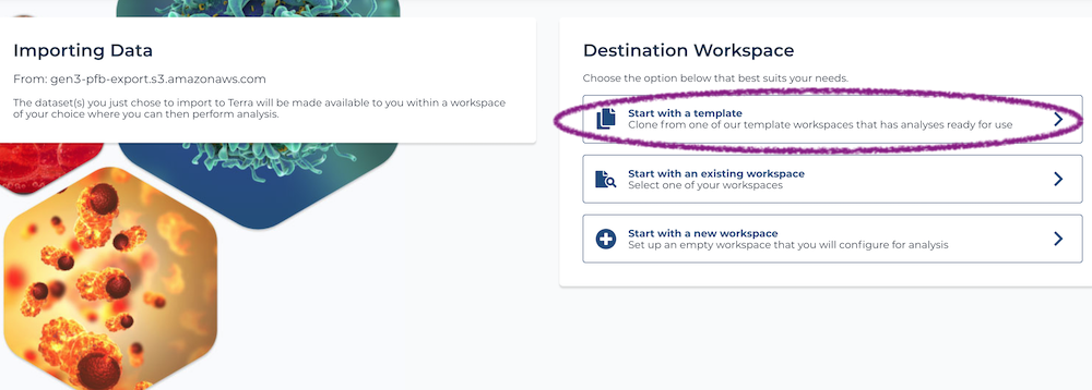
Once the new Terra window appears, you are given a few options for where to place your data.

1) "Start with a template" This feature allows you to import data directly into a template workspace that has everything set up for you to do an analysis but does not contain any data. Once you select a workspace, you will need to enter:

• Workspace name: Enter a name that is meaningful for your records.

• Billing Project: Select the billing projects available to you.

• Authorization Domain: Assign the authorization domain that you generated above to protect your data. This is important for working with controlled access. data.

2) "Start with an existing workspace" If you have already created a workspace, you can import your data directly to this workspace.

3) "Start a new workspace" This will create an empty workspace. You can individually copy notebooks and workflows from other workspaces, import workflows from Dockstore, or start fresh.

Part 2: Explore TOPMed data in Jupyter Notebooks

2a) Extract multi-sample VCFs to your workspace

Gen3 uploaded tar compressed bundles, as they are provided by dbGAP, into cloud buckets owned by BDC. To make these tar files actionable and ready for use in analyses, users will need to unarchive these tar bundlers to their workspace.

First, open the 1-unarchive-vcf-tar-file-to-workspace notebook and follow the steps to select which tar bundle(s) to extract to your workspace for use in the GWAS. Please understand that this step may be time consuming since TOPMed multi-sample VCF files are several hundred gigabytes in size.

2b) Prepare your phenotypic and genotypic data for input into association test workflows

Now that you can interact with the Gen3 structured data more easily, you will use an interactive notebook to explore your phenotypic and environmental data and performs several analyses to prepare the data for use in batch association workflows.

1. to work with the data you imported.

2. Open the 2-GWAS-preliminary-analysis notebook and set your runtime configuration. We have given a suggested configuration within the notebook.

3. From within this 2-GWAS-preliminary-analysis notebook you can call functions from the companion terra_data_table_util notebook to reformat multiple data tables into a single data table that can be loaded as a dataframe in the notebook.

Time and cost estimate

You can adjust the runtime configuration to fit your computational needs in the Jupyter notebook. We recommend selecting the default environment and selecting the custom profile to use and configure the spark cluster for parallel processing. Using the profile suggested profile within the Jupyter notebook and a project with around 1000 samples, running this notebook on this dataset takes about 90 minutes and $20/hr to compute.

When working in a notebook with computing times over 30 minutes, learn more about Terra's and for your needs. Please carefully consider how adjusting auto-pause can remove protections that help you from accidentally accumulating cloud costs that you did not need.

Part 3: Perform mixed-model association tests using workflows

In Part 2, we explored the data we imported from Gen3 and performed a few important steps for preparing our data for association testing. We generated a new "sample_set" data table that holds the files we created in the interactive notebook. These files will be used in our batch workflows that will perform the association tests. Below, we describe the four workflows in this workspace and their cost estimates for running on the sample set we create in this tutorial.

The workflows used in this template were imported from and their parameters were configured to work with Terra's data model. If you're interested in searching other Docker-based workflows, .

Notes on how attributes are set in workflows

We have set the input and output attributes for each workflow in this template. Before running the first workflow, you can look through the inputs and outputs of each workflow and see that outputs from the first workflow feed into the second workflow, and so on.

In the 2-GWAS-preliminary-analysis notebook, we created a Sample Set data table that holds a row called "systolicbp" which contains the input files for the following workflows. You can check this data table out in the Data tab of this workspace. When you open a workflow, make sure that "Sample Set" is set and the "systolicbp" (or whatever you named your run) is selected before running a workflow.

1-vcfToGds

This workflow converts genotype files from Variant Call Format () to Genomic Data Structure (), the input format required by the R package GENESIS.

Time and cost estimates

Inputs:

• VCF genotype file (or chunks of VCF files)

Outputs:

• GDS genotype file

2-genesis_GWAS

This workflow creates a null model from phenotype data with the GENESIS biostatistical package. This null model can then be used for association testing. This workflow also runs single variant and aggregate test for genetic data. Implements Single-variant, Burden, SKAT, SKAT-O and, SMMAT tests for Continuous or Dichotomous outcomes. All tests account for familiar relatedness through kinship matrixes. Underlying functions adapted from: Conomos MP and Thornton T (2016). GENESIS: GENetic EStimation and Inference in Structured samples (GENESIS): Statistical methods for analyzing genetic data from samples with population structure and/or relatedness. R package version 2.3.4.

Time and cost estimates

Inputs:

• GDS genotype file

• Genetic Relatedness Matrix

• Trait outcome name

Outputs:

• A null model as an RData file

• Compressed CSV file(s) containing raw results

• CSV file containing all associations

Cost Examples

Below are reported costs from using 1,000 and 10,000 samples to conduct a GWAS using the BioData Catalyst GWAS Blood Pressure Trait template workspace. The costs were derived from single variant tests that used Freeze 5b VCF files that were filtered for common variants (MAF <0.05) for input into workflows. The way these steps scale will vary with the number of variants, individuals, and parameters chosen. TOPMed Freeze 5b VCF files contain 582 million variants and Freeze 8 increases to ~1.2 billion. For GWAS analyses with Freeze 8 data, computational resources and costs are expected to be significantly higher.

These costs were derived from running these analyses in Terra in June 2020.

Optional: Bring your own data

Both the notebook and workflow can be adapted to other genetic datasets. The steps for adapting these tools to another dataset are outlined below:

Update the data tables Learn more about uploading data to Terra . You can use functions available from the terra_data_table_util companion notebook to consolidate new data tables you generate.

Update the notebook Accommodating other datasets may require modifying many parts of this notebook. Inherently, the notebook is an interactive analysis where decisions are made as you go. It is not recommended that the notebook be applied to another dataset without careful thought.

Run an additional workflow You can search for available workflows and export them to Terra following .

Helpful resources to master this tutorial

• If you are new to BDC-Terra, we have created an that includes several introductory webinars.

Authors, contact information, and funding

This template was created for the project in collaboration with the at and the at . The association analysis tools were contributed by the .

Contributing authors include:

• (UC Santa Cruz Genomics Institute)

• Michael Baumann (Broad Institute, Data Sciences Platform)

• Brian Hannafious (UC Santa Cruz Genomics Institute)

Workspace change log

This page is an open access preview of the Terra tutorial workspace that you can find at this link.

GWAS Tutorial in BDC

This tutorial workspace offers example tools for conducting mixed-models GWAS from start to finish using the NHLBI BioData Catalyst ecosystem. We've created a set of documents to get you started in the BioData Catalyst system. If you're ready to conduct an analysis, proceed with this dashboard:

Data Model

This template was set up to work with the NHLBI BioData Catalyst Gen3 data model. In this dashboard, you'll learn how to import open access data from the Gen3 platform into this Terra template and conduct an association test. If you have never used the Gen3 data model before, we suggest you start with the tutorial .

For this tutorial, we are using synthetic phenotypic data coupled with downsampled 1000 Genomes data that has been ingested into BDC Powered by Gen3 (BDC-Gen3). This data model is likely new to most users and may take some time to become accustomed to. First, the data model is based on a graph structure that is more complex than a single columns x rows data table that you may be familiar with. Second, genomic data is accessible through DRS URLs that point to Google Cloud Buckets that hold the data.

After this tutorial, you can employ the BDC ecosystem for more analyses. Currently, BDC-Gen3 hosts the program, which is controlled access. To apply for access to TOPMed, submit an application through .

If you already have access to a TOPMEd project and have been onboarded to the BDC platform, you should be able to access your data through BDC-Gen3 and use your data with another GWAS resource we have created that you can access .

About the data

To demonstrate an analysis that could be run on typical whole genome sequence data, this workspace provides mock phenotype data generated from publicly available 1000 Genomes phase 3 genotypes. Phenotypes have been simulated based on individual genotypes and known associated loci for multiple complex traits. The GCTA software⁶ was used with lists of causal variants and an estimate of narrow sense heritability⁵ for each phenotype.

Traits and sources for causal variants a. BMI: Giant-UKBB meta-analysis² b. Fasting glucose: MAGIC³ c. Fasting insulin: MAGIC³ d. Waist-to-hip ratio: GIANT-UKBB meta-analysis² e. Height: GIANT-UKBB meta-analysis² f. HDL: MVP⁴ g. LDL: MVP⁴ h. Total cholesterol: MVP⁴ i. Triglycerides: MVP⁴

Generating the synthetic data The scripts used to create the phenotype data, as well as intermediate data files and a readme file, are in a public Google bucket (gs://terra-featured-workspaces/GWAS/data_processing/). To browse the Google bucket, click here.

Tutorial outline

Part 1: Navigate the BDC environment Learn how to search and export data from Gen3 and worfklows from Dockstore into a Terra workspace.

Part 2: Reformat Gen3 phenotypic data for use in downstream analysis Review the data you imported in Terra and use the interactive Jupyter notebook 1-Prepare-Gen3-data-for-exploration to consolidate several clinical data tables into a single data table that can be used in the next notebook. This notebook calls functions in the companion notebook terra_data_table_util.

Part 3: Data exploration and preparation The 2-GWAS-preliminary-analysis notebook will lead you through a series of steps to explore the phenotypic and genotypic data and prepare files for import into association workflows. This is the most time and resource consuming analysis in the GWAS.

Part 4: Perform mixed-model association tests using workflows Next, perform mixed models genetic association tests (run as a series of batch workflows using GCP Compute engine). The workflows are also publicly available in in this .

Part 1: Navigate the BDC ecosystem

1a. Link your Terra account to Gen3 using external services

Before you're able to access genomic data from Gen3 in the Terra data table, you need to link your Terra account to external services. Link your profile .

1b. Create an Authorization Domain to protect your controlled-access data

If you bring controlled access data into Terra, it should be registered under an Authorization Domain that limits its access to only researchers with the appropriate approvals. Learn how to set up an Authorization Domain .

1c. Export the training dataset from Gen3 to Terra

1. Start by learning about Gen3's graph-structured data model for BDC using this .

2. Once you better understand the graph, log into through the NIH portal using your eRA Commons username and password.

3. Navigate to the view to see what datasets you currently have and do not have access to. On the left hand side, you can use the faceted search tool to narrow your results to specific projects.

1d. Select a Terra workspace for your data

Once the export window in Gen3 transitions to Terra, you are given a few options for where to place your data:

1) "Start with a template" This feature allows you to import data directly into a template workspace that has everything set up for you to do an analysis but does not contain any data. Once you select a workspace, you will need to enter:

• Workspace name: Enter a name a name that is meaningful for your records.

• Billing Project: Select the billing projects available to you.

• Authorization Domain: Assign the authorization domain that you generated above to protect your data. This is important for working with controlled access. data.

2) "Start with an existing workspace" If you have already created a workspace, you can import your data directly to this workspace.

3) "Start a new workspace" This will create an empty workspace. You can individually copy notebooks and workflows from other workspaces, import workflows from Dockstore, or start fresh.

Part 2: Reformat Gen3 phenotypic data for use in downstream analysis

If you have not used the Gen3 data model before, we recommend you first start with this tutorial and then come back to this step in the GWAS.

1. Once data has been successfully uploaded to your Terra account, review the Data tab of your Terra workspace. The tutorial dataset should include the following clinical data tables that you will use in the GWAS: Subject, Demographic, Lab Result, Sample.

2. Navigate to the Notebooks tab and open 1-Prepare-Gen3-data-for-exploration. This notebook consolidates the clinical data tables mentioned in step 1 into a single data table that can be used in the GWAS. This notebook calls functions in the companion notebook terra_data_table_util. You don't have to open terra_data_table_util notebook, it is available for users to edit for other use cases.

Note: This consolidated_metadata table is closer to the data model you use in our "Featured Workspaces". We hope these two notebooks (1-Prepare-Gen3-data-for-exploration, terra_data_table_util) help you use Gen3 data with more of our training resources in Terra.

Part 3: Explore TOPMed data in Jupyter Notebooks

Now that you can interact with the Gen3 structured data more easily, you will use an interactive notebook to explore your phenotypic and environmental data and performs several analyses to prepare the data for use in batch association workflows.

1. to work with the data you imported. Your computing needs will vary depending on the size of your VCF file.

2. Open the 2-GWAS-preliminary-analysis notebook and set your runtime configuration. We have given a suggested configuration within the notebook for a downsampled VCF (representing chromosomes 10 and 11) that we include for training purposes.

3. Call functions from the terra_data_util notebook to reformat multiple data tables into a single data table that can be loaded as a dataframe in the notebook.

Note: VCF files you import from Gen3 are in the Reference_File node and are accessible via DRS URLs. For TOPMed Freeze 5b datasets, these are also tar compressed. We have this GWAS tutorial that has notebooks and examples for interacting with these VCFs .

Time and cost estimate

Time to execute all the commands is ~28 minutes which currently costs ~$0.50 to complete (with the recommended cluster configuration available inside the notebook).

Part 4: Perform mixed-model association tests using workflows

In Part 3, we explored the data we imported from Gen3 and performed a few important steps for preparing our data for association testing. We generated a new "sample_set" data table that holds the files we created in the interactive notebook. These files will be used in our batch workflows that will perform the association tests. Below, we describe the four workflows in this workspace and their cost estimates for running on the sample set we create in this tutorial.

The workflows used in this template were imported from and their parameters were configured to work with Terra's data model. If you're interested in searching other docker-based workflows, .

Notes on how attributes are set in workflows

We have set the input and output attributes for each workflow in this template. Before running the first workflow, you can look through the inputs and outputs of each workflow and see that outputs from the first workflow feed into the second workflow, and so on.

In the 2-GWAS-preliminary-analysis notebook, we created a Sample Set data table that holds a row called "tutorial-analysis" which contains the input files for the following workflows. You can check this data table out in the Data tab of this workspace. When you open a workflow, make sure that "Sample Set" is set and the "tutorial-analysis" (or whatever you named your run) is selected before running a workflow.

1-vcfToGds

This workflow converts genotype files from Variant Call Format () to Genomic Data Structure (), the input format required by the R package GENESIS.

Time and cost estimates

Inputs:

• VCF genotype file (or chunks of VCF files)

Outputs:

• GDS genotype file

2-genesis_GWAS

This workflow creates a null model from phenotype data with the GENESIS biostatistical package. This null model can then be used for association testing. This workflow also runs single variant and aggregate test for genetic data. Implements Single-variant, Burden, SKAT, SKAT-O and SMMAT tests for Continuous or Dichotomous outcomes. All tests account for familiar relatedness through kinship matrixes. Underlying functions adapted from: Conomos MP and Thornton T (2016). GENESIS: GENetic EStimation and Inference in Structured samples (GENESIS): Statistical methods for analyzing genetic data from samples with population structure and/or relatedness. R package version 2.3.4.

Time and cost estimates

Inputs:

• GDS genotype file

• Genetic Relatedness Matrix

• Trait outcome name

Outputs:

• A null model as an RData file

• Compressed csv file(s) containing raw results

• CSV file containing all associations

Optional: Bring your own data

Both the notebook and workflows can be adapted to other genetic datasets. The steps for adapting these tools to another dataset are outlined below:

Update the data tables Learn more about uploading data to Terra .

Update the notebook Accommodating other datasets may require modifying many parts of this notebook. Inherently, the notebook is an interactive analysis where decisions are made as you go. It is not recommended that the notebook be applied to another dataset without careful thought.

Run an additional workflow You can search for available workflows and export them to Terra following .

Authors, contact information, and funding

This template was created for the project in collaboration with the at and the at . The association analysis tools were contributed by the .

Contributing authors include:

• (UC Santa Cruz Genomics Institute)

• Michael Baumann (Broad Institute, Data Sciences Platform)

• Brian Hannafious (UC Santa Cruz Genomics Institute)

Workspace change log

Onboarding Webinars

For the latest training webinars, view the recordings of our first onboarding webinar - with a data-focused agenda - and our second onboarding webinar - with an agenda covering more advanced workflow concepts such as configuration and WDL scripts.

End-to-End Workspace-Based Tutorials

These hands-on tutorials cover the full flow of selecting data in Gen3, then handing off that data to Terra for analysis.

PIC-SURE Tutorials in Terra

These workspaces hit the PIC-SURE API that offers search features for controlled-access data from BDC. You can query studies and subset based on patients matching specified criteria, as well as retrieve a cohort that has been created using the .

Additional Tutorial Articles

Additional Tutorial Resources

These tutorials often use Terra’s data model. If you would like to use Gen3 data with these examples, we suggest that you begin with , which can help you transform graph-structured data into a data model easier to use with our entire suite of tutorials.

Overview

This document is an open access preview of the Terra tutorial workspace that you can find here.

In this tutorial, you will be running the TOPMed alignment workflow as you learn how to use BDC-Terra, BDC Powered by Dockstore (BDC-Dockstore), and BDC-Gen3. This beginner-oriented tutorial walks you through how each of these platforms interact with one another.

The workflow in this tutorial is the TOPMed aligner. This workflow is a containerized version of the pipeline University of Michigan developed to process all CRAM files available in the TOPMed program. You can use this aligner workflow to prepare data for comparison with TOPMed CRAM files.

Data Models Covered in this Tutorial

One aim of this tutorial is to help you learn the Gen3 data model for TOPMed and how to interact with it. This can help you bring your own data to the BDC platform and compare it with the TOPMed data that is currently hosted in this system.

You will learn how to import TOPMed data from Gen3, which uses a more complex graph-based data model than the data model used for what's already hosted on Terra, such . However, in order to use TOPMed data from Gen3, you must be approved to use TOPMed data via . If you do not have dbGaP access, do not worry -- you will still be able to run this workflow on 1000 Genomes Data, as long as you have an NIH credential such as that can get you into Gen3.

Cost Estimate

Your costs may vary depending on how your data is formatted and what parameters you use. In addition, if you are using preemptibles, there is some element of randomness here -- a preemptible may or may not be stopped by Google at any given time, causing an in-progress task to need to restart.

When running the aligner workflow on 10 full-size CRAMs from the PharmaHD study imported from Gen3, using the aligner's default settings, the cost was $80.38 as reported by Terra. The most expensive of those ten files cost $10.82 and the least expensive cost $5.74.

Setting Up

Because Gen3 hosts controlled-access data, you will need to set up your Terra account for the linkage to Gen3 to work properly. Please see .

If you are planning to work with controlled access data, you should set up an Authorization Domain to protect your work. This will prevent you from inadvertently sharing data that shouldn't be shared. Learn more in this .

Using Gen3

If you are new to using Gen3 and Terra, you may want some background information. A good overview can be found in , which will introduce you to the Gen3 data model and how it is stored in Terra. Those seeking more specific information may want to use the following resources:

Head on over to and log in by clicking "Profile" in the top right hand corner. You will need to log in using your NIH eRA Commons ID. When you click on "Exploration" you will see all subjects and studies you have access to. Use filters on the right hand side of the screen to select what you are interested in.

Selecting by study/project

If you are interested in a particular study, click the "subject" tab on the leftmost toolbar. You will see a dropdown menu to select by project ID. In this example, we will search by Project ID for "1000 Genomes".

Importing to Terra

After selecting a project, click the red "Export To Terra" button. Bear in mind that exporting may take a few minutes and you shouldn't navigate away from the page while this is happening. Once it completes, you will be taken to a Terra page where you can choose which workspace to put your data into. From here, you should select "template workspace" and import into the TOPMed aligner workspace.

What happens next? A copy of this exact workspace will be created, with several data table that hold administrative, and any clinical and biospecimen data associated with the project. Biospecimen data tables will hold DRS that point to the location of the genomic data hosted by NHLBI. You can learn more about DRS . It will take a few minutes for the data to fully import, but once it does, you'll see the workspace has been populated with several data tables.

One of the data tables you'll see is called "Submitted Aligned Reads." If you scroll across that in Terra's UI, you will see a column named "data_format," indicating that these are CRAM files. But where are those files actually? Keep scrolling and you will see "pfb:object_id" as a column header, and under that, several drs:// URIs. This is what Terra will be using to locate the files. Thankfully, you don't need to remember these URIs. When running a workflow, if we want to run a WDL on this data, we can reference that pfb:object_id column in order to enter dozens (hundreds, even) of URIs into a workflow with just a few clicks.

Running the Aligner

The links at the top of this section should serve as an explanation as to how Gen3 data is stored. But even with that background, it may still look a little odd when imported into Terra, so let's walk through how to use these tables. If you want a more complete explanation of how these tables relate to each other, see the optional section towards the end of this workspace.

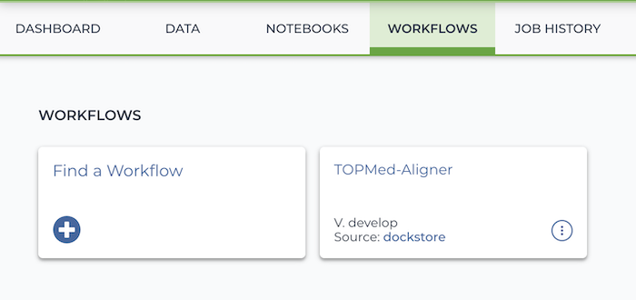
Select this workspace's Workflows tab. You will see a WDL has already been imported from Dockstore: a Dockerized version of the . Select it.

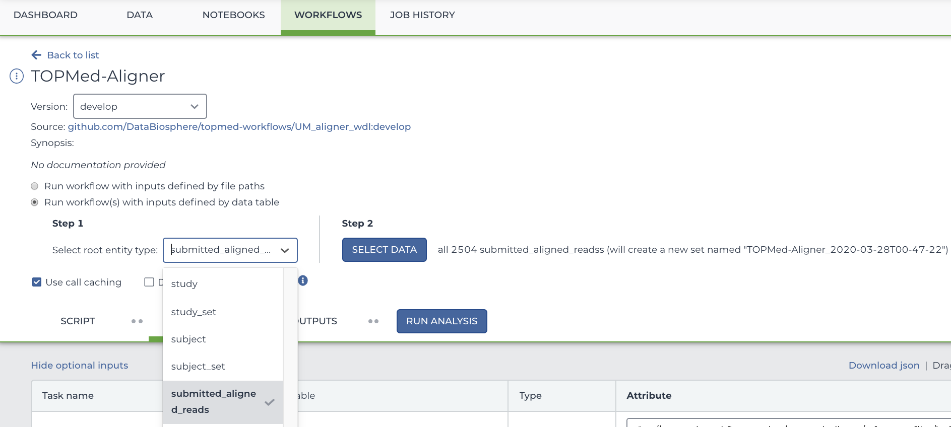
You will see two buttons. Select the bubble labeled "Run workflow(s) with inputs defined by data table", and in the drop down menu, select "Submitted Aligned Reads".

To select only particular participants, click "Select Data" which is located to the right of the Step 2 heading. This will open a new menu where you can select precisely which rows you want to run your workflow on. In this case, each row represents a participant.

Below this, you will see several arguments that can be used for this workflow. If it's not already filled out, type out this.pfb:object_id as the input_cram_file.

But what is "this"? In Terra, we can use "this" to represent the data table that we selected from the drop down menu. So, in this case, "this" refers to the Submitted Aligned Reads data table. As for ".pfb:object_id", that part means that Terra is looking at the column called "pfb:object_id" in said data table.

For more information on using workflow inputs on Terra, please see

To Preempt or Not to Preempt?

If you already know what preemptibles are and don't want to use them, you can skip this section, as this template workspace is set up to avoid them by default.

When computing on Google Cloud, you have the option of using preemptible virtual machines. These virtual machines work essentially the same as what you expect from Google Cloud, but they are significantly cheaper (sometimes less than half the price!). There is a catch, however -- they may shut down in the middle of a task and only exist for 24 hours at most. You can find more information , but let's talk about the specifics of this workspace.

This isn't a concern if you were running on small test CRAM files such as the ones on the aligner's Dockstore sample JSON. But when running on full-size CRAM files such as ones imported from Gen3, there is a chance that any given step (pre-alignment, alignment, or post-alignment) might get shut down before it completes if it's run on a preemptible VM. This is especially true of the post-align step, which tends to take the longest, often more than 24 hours when running on full-sized CRAM files.

We've broken down some possibilities here so you can balance risk, run time, and cost:

Whenever preemptible_tries is a positive integer, the task will exhaust all preemptible tries before trying on the more expensive non-preemptible VM. The same logic applies for PreAlign_preemptible_tries and PreAlign_max_retries, as well as Align_preemptible_tries and Align_max_retries. Terra handles all this on its own; you don't have to manually restart any of these tasks as long as the workflow itself is still running.

Once you have decided if you want to change the default behavior for preemptible VMs, press "save" and run your workflow.

Tracking the Aligner's Progress

With your workflow now running, click on the "JOB HISTORY" tab at the top of this workspace. You will see a table detailing every submission you have made in your workspace.

Let's click on the top row, which shows the most recently submitted workflow. You will see something like this -- metadata on the top, and below that, a one-row table. If you click on "view" in the leftmost tab of the table (marked with a square below), you will more information about the workflow, including how long it's running certain tasks. In this case, that means pre-alignment, alignment, and post-alignment. This can come in handy of a workflow fails, as this screen will tell you how long each task has run for, how many attempts it had, and (if applicable) any logs created in the process. You can also click "workflow ID" in the leftmost column (circled) to be taken to Google Cloud's own website to explore the bucket, although you can do the same on Terra itself.

Take note of the submission ID and workflow ID, or at least the first few digits of each. They'll come in handy in a moment.

Examining Output

As the aligner does its thing, it will begin writing files to the Google Cloud bucket your workspace is hosted on. You can find this in the "Files" section of your workspace's DATA tab. Note that this "Files" section will be the lefthand side below all of the data tables you imported from Gen3, so you'll probably have to scroll a bit to see it.

Remember that workflow ID we took note of earlier? That workflow ID is also the name of the folder that your workflow is writing to. Keep in mind every time you run a workflow, a new folder will be created, even if you are just running the same workflow on the same data with the same parameters. In your workspace's file system, your output data for the aligner will be stored in Files/{submission ID}/TopMedAligner/{workflow ID}/call-PostAlign/. So, for instance, in the screenshot above my submission ID started with "b17b9937-ff17-46e8-b20b-798dc3d4ebf2" and my workflow ID started with "2368abf3-0e2a-4cd7-b10a-89d4d1f9002d." So my output files are located in Files / b17b9937-ff17-46e8-b20b-798dc3d4ebf2 / TopMedAligner / 2368abf3-0e2a-4cd7-b10a-89d4d1f9002d / call-PostAlign /. Of course, these files will only be created once the aligner finishes -- if your workflow is running but hasn't finished yet, the call-PostAlign folder might not exist yet.

Running on More Than One Data Table

This is optional to run the aligner included in this workspace, however, certain other workflows may require you to draw upon more than one table, so this is good information to learn.

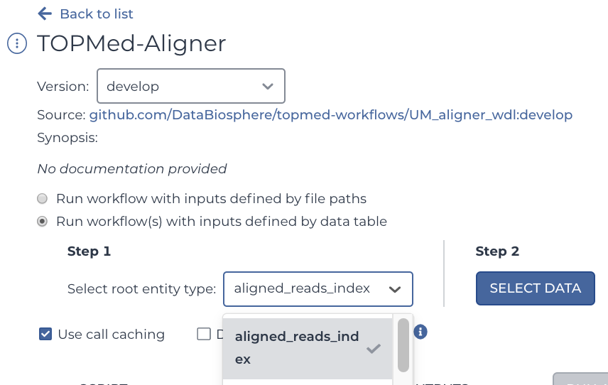
Go back to the workflow tabs and again select the aligner. However, this time, select "Aligned Reads Index" instead of "Submitted Aligned Reads". Yes, this is a table of CRAI files, not CRAM files -- but like the CRAM table, it too links to its files using DRS URIs in the pfb:object_id column. Don't worry, we'll get back to the CRAMs in a moment.

Like what was indicated in the section detailing Gen3's data structure, your input will depend on what table you select. In our case, we selected Aligned Reads Index. So that means that now anything that says "this" for an input will be looking at the Aligned Reads Index table.

In this version of the TOPMed aligner, CRAI files optional, but for the sake of learning more about Gen3's data structure we will be using them. In Gen3's data structure, CRAI files are considered a child of CRAM files, or in other words, "submitted aligned reads" table (which includes the CRAM files and their metadata) is the parent of "aligned reads index" table (the CRAI files and their metadata). When dealing with Gen3 data, children know their parents, but not vice versa. In summary, the table containing CRAI files also links to the table that contains CRAM files, but not vice versa. In this particular example, that link is stored in the CRAI table as a column named submitted_aligned_reads. Note that it does not link to the table overall, but rather a given row of that table: Each row on the CRAI table points to the row of the CRAM table that its associated with. This can be a bit confusing to wrap your head around, so feel free to click through your data tables on Terra or review Gen3's documentation if you're getting a headache at this point.

Why does this matter? Because you can use this to effectively use two different data tables in your analysis, even though at first glance it looks like you can only select one in the drop down menu. You simply enter that table's link to the CRAI files, ie, this.pfb:object_id as the input for input_crai_file. (You will have to scroll to find input_crai_file in the aligner as Terra puts optional arguments below all required arguments.) And for input_cram_file, the correct entry is this.submitted_aligned_reads.pfb:object_id. Handy, isn't it?

Final Notes

We have now gone over how to set up the TOPMed alignment workflow to work with the Gen3 graph-model. Below are some final notes if you want to align your data from other sources using this workflow.

• -- useful if you want to preform further analysis on your newly aligned data

If Your Data Was or Will Be Aligned to Something that Isn't HG38

Something that may be easy to miss in the aligner's documentation is the following note:

The CRAM to be realigned may have been aligned with a different reference genome than what will be used in the alignment step. The pre-align step must use the reference genome that the CRAM was originally aligned with to convert the CRAM to a SAM.

There are two important things to take away from this:

1. If what you already aligned your data to (remember, CRAM/SAM/BAM files are already aligned) does not match the reference genome you are aligning to with this workflow, you must include what you aligned them to as the argument for PreAlign_reference_genome and its associated index as the argument for PreAlign_reference_genome_index. For instance, if your CRAM files were generated using HG19 as your reference and you are using this workflow to align them HG38, you must set HG38 as your argument for ref_fasta and HG19 as PreAlign_reference_genome.

2. TOPMed data is aligned to HG38. If you are running this workflow to compare your own data to TOPMed data, you must align to HG38.

Authors

Workspace author: Ash O'Farrell WDL script and bug fixing: Walt Shands Dockerized TopMED Aligner: Jonathon LeFaive Edits and bug-squashing: Michael Baumann, Beth Sheets

This workspace was completed under the BDC project.

Workspace Changelog